Elementary Information Theory for Neuroscience
This is a slightly modified version of an article I wrote for a neural computation class I took at Berkeley. There were a few people who found it intriguing, so I thought I’d post it on my blog for anyone else who could be interested. It shouldn’t require too much of a background in either statistics or neuroscience, but I do exclude some definitions that you can quickly look up on DuckDuckGo. The basics of information theory are quite simple and its reach extends to almost every field in STEM, and I personally find it to be quite a beautiful topic.
Motivation
What is information theory and why is it relevant to neuroscientists? At its core, information theory is about the limits of how information can be communicated efficiently. We will develop a more explicit definition of information soon, but for now think of information as any sort of knowledge about the world. Why would this be relevant to neuroscientists? At a high level, the brain can be thought of as a “thing” that represents and manipulates information in order to make decisions. But representing and manipulating this information is not free, it comes at the cost of energy. If this cost is too expensive, the organism will likely die. So we would expect natural selection to select for brains that are relatively efficient at this process of representing and manipulating information. Therefore information theory can give us a valuable framework to think about possible ways the brain could be organized. In order to do so, however, we must first define some of the basic ideas in information theory.
Basics of Information Theory
While we may have an intuitive idea about what information is, coming up with a mathematical formulation of that idea can be challenging. To do so, we will start with a term known as the entropy of a random variable $X$. Note that much of information theory is built off of the framework of statistics, so if you are unfamiliar with a term such as a random variable, just do a quick internet search. Broadly speaking, the entropy of a variable is the amount of uncertainty that a variable contains. Formally, we write that the entropy of a variable $X$, $H(X)$, is defined as:
\[H(X) = \sum_{i = 1}^{n}p(x_i) \cdot log_2(\frac{1}{p(x_i)})\]But let’s break this down to more than just mathematical jargon. We said that the entropy is meant to quantify the amount of uncertainty in a variable. How does this term do so? Say that $X$ represents the random variable of whether or not it will rain tomorrow. Now say that $P(X)$, the probability distribution of X, is that it will rain with probability 0.01 and will not rain with probability 0.99. We can be fairly confident that it will likely not rain tomorrow, that is to say we don’t have much uncertainty. But what if it did rain tomorrow? We would be rather surprised! How can we quantify this surprise? One way to possibly do it would be to look at the inverse probability, $\frac{1}{p(x)}$. So in our previous example, if it rained we would have 100 units of surprise, and if it didn’t rain we would have ~1 unit of surprise. The latter fact seems a bit weird though, especially considering that if we knew for certain that it wasn’t going to rain tomorrow, we would still have $\frac{1}{1} = 1$ unit of surprise when it doesn’t in rain. So we can do a log transform and instead define the surprise as $log(\frac{1}{p(x)})$. Doing so gives us the following graph of how “surprised” we are:
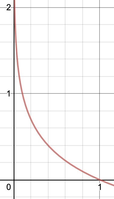
This plot of surprise makes a lot more sense. If we know an event will definitely happen, i.e. if the probability is 1, then we have 0 surprise that the event happened. Alternatively, as the probability that an event happens approaches 0, we become more and more surprised if it does happen. Using this idea, we can now look at the entropy as :
\[H(X) = \sum_{all\ events\ x_i}p(event\ x_i\ occurs) \cdot surprise(event\ x_i\ occurs)\] \[H(X) = E_x[surprise(x_i\ occurs)]\] \[H(X) = E_x[log_2(\frac{1}{p(x)})]\]So what is entropy? It is nothing more than the weighted sum of how surprised we are by each event occurring (note that here we write it the way it tends to be written in literature, which replaces the summation with something equivalent in statistics called an expectation) This seems like a pretty good definition of uncertainty!
How does this definition of entropy help us with defining information? One way to look at information is as a quantity that reduces uncertainty. For example, imagine that we somehow know that it will rain on either Saturday or Sunday this week, each with their own probability. We also know that for whatever reason, it won’t rain on both days. Saturday comes around and it doesn’t rain. Using this information, we know that it will definitely rain on Sunday since it didn’t rain on Saturday. Phrasing this another way, we have reduced our uncertainty about whether or not it will rain on Sunday using the information that it didn’t rain on Saturday. Formally, we call this the mutual information between two events, and it is defined as:
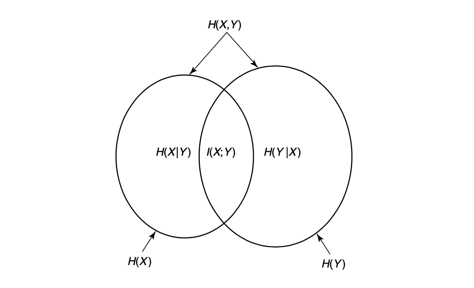
\[I(X;Y) = H(X) - H(X|Y)\]Again, let us try to understand the intuition behind this mathematical notation. Given two events $X$ and $Y$, we have some amount of uncertainty about them both, $H(X)$ and $H(Y)$, respectively. The mutual information is how much less uncertain we are about $X$ given that we know $Y$. To put it another way, it is the amount of uncertainty shared by both $X$ and $Y$. For a nice visual of this relationship, see the diagram below [2].
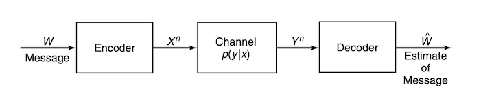
The last important concept from information theory that we will introduce is called capacity. For this we will also have to introduce the notion of a channel, which you can think of as a cable. For example, I could connect my laptop to an external monitor via a HDMI cable. To see how this relates to the idea of a channel, a diagram of a general channel is shown below [2]. You can think of $W$ as your laptop, the channel as the cable, and $\hat{W}$ as the external monitor. For now we won’t say much about the Encoder and Decoder other than that they are a way to transform the input and output of the channel. The value of this will hopefully be clear after a bit more explanation.
Ideally I would like all of the data from my laptop to be perfectly transmitted to the monitor so that I can have a clear image of what I’m working on. Unfortunately, much like anything else in the world, the cable (more generally, the channel) will likely add noise that could disrupt our data. How do we deal with this and recover our original data? Here is where the concept of capacity comes into play. A channel’s capacity is the maximum amount of information that it can convey. Formally, we define this as:
\[C = \max_{p(x)} I(X;Y)\]Once again, let’s try to establish the intuition behind this. In a vacuum, we would not know anything about what should be on the external monitor. It could be a cat, a solid purple screen, or this very article. But given that we know what image the laptop is trying to transmit, we should be less uncertain about what the monitor should display. As we just discussed, this reduction of uncertainty is precisely the mutual information. Then we want to maximize this information between the monitor and the display so that we can get a clear picture! How can we maximize it? Here is where the Encoder comes into play. We want to choose an encoding of the input that is able to minimize the amount of noise that is added by the cable. To find a particular encoding, many different optimization frameworks can be used depending on the problem. The important intuition to take away is that the encoding allows us to transform the input in a way that maximizes the amount of information we can communicate over the channel, with the decoder playing a similar and opposite role.
Some Applications to Neuroscience
Now that we have the building blocks of information theory down, we turn to some of their applications to neuroscience.
We start with the information capacity of a neuron. One of the main ways that neurons convey information is via electrical signals called spikes, which is what we will focus on for this analysis. One way to think about neural spikes in terms of everyday objects is as a simple on-off switch that resets to the off position shortly after being switched on. The information capacity of a neuron is then based on the ability to convey information via different messages, which amounts to how many different ways we can generate patterns of turning the switch on in some given interval of time. Using neuroscience terms, we would call this generating different spike trains. Therefore if a neuron has a mean firing rate of $R$ and is trying to spike within $T$ different intervals, we can use basic combinatorial analysis to show that there are $T \choose R$ different ways to do so [1]. Using this, we can then compute the information that a neuron can convey by computing a quantity called the self-information:
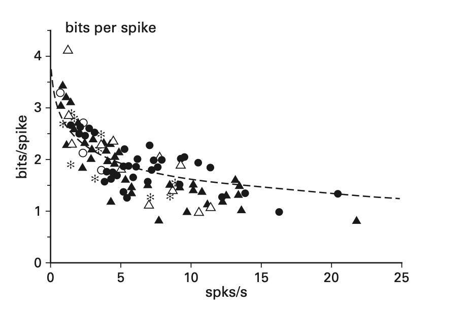
\[I(X;X) = H(X) - H(X|X)\] \[I(X;X) = H(X)\] \[I(X;X) = log_2(\frac{T!}{R!(T-R)!})\] \[I(X;X) = log_2(T!) - log_2(R!) - log_2((T-R)!)\]We can plot this equation to notice that information per spike increases sub-linearly with neuron firing rate. So the more often the neuron is spiking, the less efficient it is overall. From this analysis we arrive at a basic principle. To maximize efficiency, neurons should fire as infrequently as possible while still being able to accurately communicate information [1]. We can think about this intuitively as the classic example of the boy who cries wolf. We are less surprised (and therefore have less information) by the boy who cries wolf every night than if Animal Protection Services came and told us to avoid the area because of a wolf. Signals that are less frequent will carry more information because we are more surprised. This is demonstrated empirically in the graph below, where we see that as the rate of spikes increases, the amount of information conveyed by each spike decreases [1]. However, there is an additional factor to account for when considering the efficiency. Because an increase in firing rate necessitates an increase in axon volume, there needs to be more energy devoted to powering the axon, which means even less efficiency. All of this leads to the conclusion that we should try to minimize the firing rate as much as possible while still building a system that can communicate accurately [1].
This intuition will be valuable when thinking about the efficient coding model of the retina. This models asks the questiton: given an image $X$ as input to the retina, how can the image be efficiently encoded and transmitted to downstream neurons in the optic nerve? Specifically, how can we think about this in light of what we previously established, with the efficiency of neurons decreasing as their firing rate increases? Let’s think about what we discussed in the section on the basics of information theory in order to do so. We have some data that we would like to communicate to another part of the brain. However, because of noise in the membrane and other signals, we cannot perfectly transmit this information. Looking at the above diagram of a channel, we can think about this process in a similar way. The image is the message that we wish to transmit, the encoder is the retina, and the channel is the optic nerve. Our goal then is to be able to communicate as much information from the image to the optic nerve as possible given the presence of noise, indicated by the various values of $n$. There is, however, one additional constraint that we previously established. We also wish to encode this data in such a way that the downstream neurons don’t need to fire too frequently, where the firing rate is indicated by $r$. A diagram of this entire model is shown below [3]. Note that our model does not include a decoder like you saw in the previous section. This is because the data is transmitted to the visual cortex, which does further processing without needing to decode the data back into its original representation.
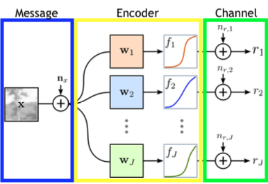
So we want to be able to transmit as much information as possible from X to R while minimizing the number of spikes that need to occur. We can write the first part of this as maximizing the mutual information between X and R, $I(X;R)$, but we haven’t yet seen a way to deal with the second part. For this we add something called a penalty term that we want to minimize, $\sum_{j} \lambda_j r_j$, where $r_j$ represents the firing rate of neuron j and $\lambda_j$ represents the cost of that firing rate. The idea here is that for some positive term $\lambda_j$, having a higher firing rate $r_j$ will have a higher cost since we are trying to minimize $\sum_{j} \lambda_j r_j $. Putting all of this together, we get the following objective function [3]:
\[\max \ I(X;R)- \sum_{j} \lambda_j r_j\]For brevity, we omit the details of how this objective is optimized. However when it is optimized, there are some pretty fascinating results. The encoding that is found is fairly simple, with each neuron in the encoder representing a small circle in the image space. This is shown in the leftmost plot below, where each square represents a different neuron and shows the learned weight $w_j$ and nonlinearity $f_j$. Further, we see that there are two types, one that is positively coding for the pixels in a localized patch, indicated with white, and one that is negatively coding for pixels, indicated with black. We call the former on-center neurons and the latter off-center neurons. Then the two rightmost plots show the result of aggregating all of on-center neurons into one plot and all of the off-center neurons into another. We see that both the on and off center neurons tile the image space quite well, with the off-center neurons being slightly smaller and more dense [3].
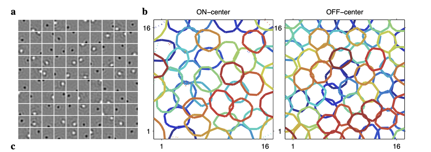
What’s so incredible about this is that it closely mimics the behavior of receptive fields in the retina. This is pretty astonishing, as we started from a purely theoretical framework, one in which we hypothesized that the brain should maximize efficient communication of information. Yet using this theoretical approach we were able to derive an information-theoretic objective that gives us a result that closely mimics biological behavior. It’s quite a remarkable finding.
This is far from the only place that information theory pops up in neuroscience. Sterling and Laughlin have a pretty epic coverage of it in their textbook that I have cited a few times throughout this post. It’s definitely one of the most interesting textbooks I have ever read, and I would highly recommend it. More broadly, information theory pops up in almost every field in STEM that I’m familiar with, as well as many social sciences that use math such as economics. It’s an incredibly valuable framework for using math to describe natural phenomenon, whether it’s complex like neural coding or simple like whether or not to bring an umbrella. If that’s not cool, I don’t know what is.
References
[1] Principles of Neural Design, Sterling and Laughlin
[2] Elements of Information Theory, Cover and Thomas
[3] Efficient coding of natural images with a population of noisy Linear-Nonlinear neurons, Karklin and Simoncelli